如何在 opencv 中仅提取 nxn 图像的 3 个特征向量?
How to extract only 3 eigen vectors of an nxn image in opencv?
我正在尝试使用以下方法将 RGB 图像转换为灰度图像 paper。
论文中使用的主要算法是这样的:
Novel PCA based algorithm to convert images to grayscale
但是,当我尝试从图像中提取特征向量时,我得到了 500 个特征值,而不是所需的 3 个。据我所知,一个 NxN 矩阵通常会给出 N 个特征向量,但我不确定我应该在这里做什么才能只得到 3 个特征向量。
关于我应该做什么的任何帮助?到目前为止,这是我的代码:
import numpy as np
import cv2

def pca_rgb2gray(img):
    """
    NOVEL PCA-BASED COLOR-TO-GRAY IMAGE CONVERSION
    Authors:
    -Ja-Won Seo
    -Seong Dae Kim
    2013 IEEE International Conference on Image Processing
    """
    I_re = cv2.resize(img, (500,500))
    Iycc = cv2.cvtColor(I_re, cv2.COLOR_BGR2YCrCb)
    Izycc = Iycc - Iycc.mean()
    eigvals = []
    eigvecs = []
    final_im = []
    for i in range(3):
        res = np.linalg.eig(Izycc[:,:,i])
        eigvals.append(res[0])
        eigvecs.append(res[1])
    eignorm = np.linalg.norm(eigvals)
    for i in range(3):
        eigvals[i]/=eignorm
        eigvecs[i]/=np.linalg.norm(eigvecs[i])
        temp = eigvals[i] * np.dot(eigvecs[i], Izycc[:,:,i])
        final_im.append(temp)
    final_im = final_im[0] + final_im[1] + final_im[2]
    return final_im
if __name__ == '__main__':
    img = cv2.imread('image.png')
    gray = pca_rgb2gray(img)
背景
当 Seo 和 Kim 要求 lambda_i, v_i <- PCA(Iycc)、i = 1, 2, 3 时,他们想要:
from numpy.linalg import eig
lambdas, vs = eig(np.dot(Izycc, Izycc.T))
对于 3×N 数组 Izycc。即他们想要Izycc的3×3协方差矩阵的三个特征值和特征向量,3×N数组(对你来说,N=500*500)
但是,由于数值不稳定性,您几乎从不想计算协方差矩阵,然后找到它的特征分解。有一个更好的方法来获得相同的 lambdas, vs,直接使用 Izycc 的奇异值分解 (SVD)(参见 this answer)。下面的代码向您展示了如何执行此操作。
给我看代码
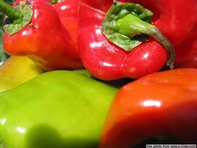
先下载http://cadik.posvete.cz/color_to_gray_evaluation/img/155_5572_jpg/155_5572_jpg.jpg并保存为peppers.jpg.
然后,运行以下内容:
import numpy as np
import cv2
from numpy.linalg import svd, norm

# Read input image
Ibgr = cv2.imread('peppers.jpg')

# Convert to YCrCb
Iycc = cv2.cvtColor(Ibgr, cv2.COLOR_BGR2YCR_CB)

# Reshape the H by W by 3 array to a 3 by N array (N = W * H)
Izycc = Iycc.reshape([-1, 3]).T

# Remove mean along Y, Cr, and Cb *separately*!
Izycc = Izycc - Izycc.mean(1)[:, np.newaxis]

# Make sure we're dealing with zero-mean data here: the mean for Y, Cr, and Cb
# should separately be zero. Recall: Izycc is 3 by N array.
assert(np.allclose(np.mean(Izycc, 1), 0.0))

# Compute data array's SVD. Ignore the 3rd return value: unimportant.
(U, S) = svd(Izycc, full_matrices=False)[:2]

# Square the data's singular vectors to get the eigenvalues. Then, normalize
# the three eigenvalues to unit norm and finally, make a diagonal matrix out of
# them. N.B.: the scaling factor of `norm(S**2)` is, I believe, arbitrary: the
# rest of the algorithm doesn't really care if/how the eigenvalues are scaled,
# since we will rescale the grayscale values to [0, 255] anyway.
eigvals = np.diag(S**2 / norm(S**2))

# Eigenvectors are just the left-singular vectors.
eigvecs = U;

# Project the YCrCb data onto the principal components and reshape to W by H
# array.
Igray = np.dot(eigvecs.T, np.dot(eigvals, Izycc)).sum(0).reshape(Iycc.shape[:2])

# Rescale Igray to [0, 255]. This is a fancy way to do this.
from scipy.interpolate import interp1d
Igray = np.floor((interp1d([Igray.min(), Igray.max()],
                            [0.0, 256.0 - 1e-4]))(Igray))

# Make sure we don't accidentally produce a photographic negative (flip image
# intensities). N.B.: `norm` is often expensive; in real life, try to see if
# there's a more efficient way to do this.
if norm(Iycc[:,:,0] - Igray) > norm(Iycc[:,:,0] - (255.0 - Igray)):
    Igray = 255 - Igray

# Display result
if True:
    import pylab
    pylab.ion()
    pylab.imshow(Igray, cmap='gray')

# Save result
cv2.imwrite('peppers-gray.png', Igray.astype(np.uint8))
这会产生以下灰度图像,似乎与本文图 4 中的结果相匹配(尽管请参阅此答案底部的警告!):
您的实施错误
Izycc = Iycc - Iycc.mean() 错误。 Iycc.mean() 展平图像并计算平均值。你想要 Izycc 这样 Y 通道、Cr 通道、 和 Cb 通道都有 zero-mean。您可以在 for dim in range(3) 循环中执行此操作,但我在上面使用数组广播执行了此操作。我在上面也有一个断言来确保这个条件成立。从数据数组的 SVD 中获得协方差矩阵的特征分解的技巧 需要 zero-mean Y/Cr/Cb 通道。
np.linalg.eig(Izycc[:,:,i]) WRONG. 这篇论文的贡献是使用主成分将颜色转换为灰度。这意味着您必须组合颜色。您在上面进行的处理是在 channel-by-channel 基础上进行的——没有颜色组合。此外,分解 500×500 数组是完全错误的:数组的 width/height 无关紧要,只有像素。出于这个原因,我将输入的三个通道重塑为 3×whatever 并对该矩阵进行操作。确保您了解 BGR-to-YCrCb 转换之后和 SVD 之前发生的情况。
与其说是错误,不如说是警告:调用 numpy.linalg.svd 时,full_matrices=False 关键字很重要:这使得“economy-size”SVD,仅计算三个 left/right 奇异向量和三个奇异值。 full-sized SVD 将尝试制作 right-singular 向量的 N×N 数组:N = 114270 像素(293 x 390 图像),float64 的 N×N 数组将是 N ** 2 * 8 / 1024 ** 3 或 97 GB。
最后的笔记
这个算法的神奇之处在于我的代码中的一行代码:
Igray = np.dot(eigvecs.T, np.dot(eigvals, Izycc)).sum(0) # .reshape...
这是数学最厚的地方,所以让我们分解一下。
Izycc是一个3×N的数组,行数为zero-mean; eigvals 是一个 3×3 对角线数组,包含协方差矩阵 dot(Izycc, Izycc.T) 的 特征值 (如上所述,通过快捷方式计算,使用Izycc),eigvecs 是一个 3×3 正交矩阵,其列是 特征向量 对应于那些协方差的特征值。
因为这些是Numpy arrays而不是matrixes,所以我们必须使用dot(x,y) for matrix-matrix-multiplication,然后我们使用sum,这两者都掩盖了线性代数。您可以自己检查一下,但上面的计算(在 .reshape() 调用之前)等同于
np.ones([1, 3]) · eigvecs.T · eigvals · Izycc = dot([[-0.79463857, -0.18382267, 0.11589724]], Izycc)
其中 · 为真 matrix-matrix-multiplication,sum 被 pre-multiplying 替换为 row-vector 个。这三个数字,
- -0.79463857乘以每个像素的Y-channel(亮度),
- -0.18382267乘以Cr(red-difference),和
- 0.11589724 乘以 Cb (blue-difference),
为这个特定图像指定“完美”加权平均值:每个像素的 Y/Cr/Cb 通道与图像的协方差矩阵对齐并求和。从数值上看,每个像素点的Y-value略微衰减,Cr-value明显衰减,Cb-value衰减更多但符号相反——这是有道理的,我们期望亮度对于灰度来说信息量最大,因此它的贡献最高。
小警告
我不太确定 OpenCV 的 RGB 到 YCrCb 的转换从何而来。 cvtColor, specifically the section on RGB ↔︎ YCrCb JPEG doesn’t seem to correspond to any of the transforms specified on Wikipedia. When I use, say, the Colorspace Transformations Matlab 包的文档只做 RGB 到 YCrCb 的转换(引用维基百科条目),我得到了一个更好的灰度图像,看起来更类似于论文的图 4:
当涉及到这些颜色变换时,我完全不知所措——如果有人能解释如何在 Python/OpenCV 中获得 Wikipedia 或 Matlab 的色彩空间变换等价物,那就太好了。尽管如此,这个警告是关于准备数据的。制作Izycc后,3×Nzero-mean数据数组,以上代码fully-specifies剩下的处理。
不幸的是,Ahmed 接受的答案有 PCA 数学错误,导致结果与手稿完全不同。这是从手稿中截取的图像屏幕。
平均居中和SVD应该沿着另一个维度进行,通道被视为不同的样本。平均居中旨在获得零的平均像素响应,而不是零的平均通道响应。
链接算法还明确指出,PCA 模型的投影首先涉及将图像乘以分数,然后将此乘积乘以特征值,而不是像其他答案那样反过来。
有关数学的更多信息,请参阅我的 PCA math answer here
可以在输出中看出代码的差异。由于手稿没有提供示例输出(我发现的),结果之间可能存在细微差异,因为手稿是捕获的屏幕截图。
为了比较,下载的彩色文件比屏幕截图的对比度高一点,因此输出的灰度也应该相同。
首先是 Ahmed 代码的结果:
然后更新代码的结果:
更正后的代码(基于 Ahmed 的以便于比较)是
import numpy as np
import cv2
from numpy.linalg import svd, norm

# Read input image
Ibgr = cv2.imread('path/peppers.jpg')
#Convert to YCrCb
Iycc = cv2.cvtColor(Ibgr, cv2.COLOR_BGR2YCR_CB)

# Reshape the H by W by 3 array to a 3 by N array (N = W * H)
Izycc = Iycc.reshape([-1, 3]).T

# Remove mean along Y, Cr, and Cb *separately*!
Izycc = Izycc - Izycc.mean(0)  #(1)[:, np.newaxis]
# Mean across channels is required (separate means for each channel is not a
# mathematically sensible idea) - each pixel's variation should centre around 0

# Make sure we're dealing with zero-mean data here: the mean for Y, Cr, and Cb
# should separately be zero. Recall: Izycc is 3 by N array.
# Original assertion was based on a false presmise. Mean value for each pixel should be 0
assert(np.allclose(np.mean(Izycc, 0), 0.0))

# Compute data array's SVD. Ignore the 3rd return value: unimportant in this context.
(U, S, L) = svd(Izycc, full_matrices=False)

# Square the data's singular vectors to get the eigenvalues. Then, normalize
# the three eigenvalues to unit norm and finally, make a diagonal matrix out of
# them.
eigvals = np.diag(S**2 / norm(S**2))

# Eigenvectors are just the right-singular vectors.
eigvecs = U;

# Project the YCrCb data onto the principal components and reshape to W by H
# array.
# This was performed incorrectly, the published algorithm shows that the eigenvectors
# are multiplied by the flattened image then scaled by eigenvalues
Igray = np.dot(eigvecs.T, np.dot(eigvals, Izycc)).sum(0).reshape(Iycc.shape[:2])
Igray2 = np.dot(eigvals, np.dot(eigvecs, Izycc)).sum(0).reshape(Iycc.shape[:2])
eigvals3 = eigvals*[1,-1,1]
Igray3 = np.dot(eigvals3, np.dot(eigvecs, Izycc)).sum(0).reshape(Iycc.shape[:2])
eigvals4 = eigvals*[1,-1,-1]
Igray4 = np.dot(eigvals4, np.dot(eigvecs, Izycc)).sum(0).reshape(Iycc.shape[:2])

# Rescale Igray to [0, 255]. This is a fancy way to do this.
from scipy.interpolate import interp1d
Igray = np.floor((interp1d([Igray.min(), Igray.max()],
                            [0.0, 256.0 - 1e-4]))(Igray))
Igray2 = np.floor((interp1d([Igray2.min(), Igray2.max()],
                            [0.0, 256.0 - 1e-4]))(Igray2))
Igray3 = np.floor((interp1d([Igray3.min(), Igray3.max()],
                            [0.0, 256.0 - 1e-4]))(Igray3))
Igray4 = np.floor((interp1d([Igray4.min(), Igray4.max()],
                            [0.0, 256.0 - 1e-4]))(Igray4))

# Make sure we don't accidentally produce a photographic negative (flip image
# intensities). N.B.: `norm` is often expensive; in real life, try to see if
# there's a more efficient way to do this.
if norm(Iycc[:,:,0] - Igray) > norm(Iycc[:,:,0] - (255.0 - Igray)):
    Igray = 255 - Igray
if norm(Iycc[:,:,0] - Igray2) > norm(Iycc[:,:,0] - (255.0 - Igray2)):
    Igray2 = 255 - Igray2
if norm(Iycc[:,:,0] - Igray3) > norm(Iycc[:,:,0] - (255.0 - Igray3)):
    Igray3 = 255 - Igray3
if norm(Iycc[:,:,0] - Igray4) > norm(Iycc[:,:,0] - (255.0 - Igray4)):
    Igray4 = 255 - Igray4

# Display result
if True:
    import pylab
    pylab.ion()
fGray =    pylab.imshow(Igray, cmap='gray')
# Save result
cv2.imwrite('peppers-gray.png', Igray.astype(np.uint8))

fGray2 = pylab.imshow(Igray2, cmap='gray')
# Save result
cv2.imwrite('peppers-gray2.png', Igray2.astype(np.uint8))

fGray3 =pylab.imshow(Igray3, cmap='gray')
# Save result
cv2.imwrite('peppers-gray3.png', Igray3.astype(np.uint8))

fGray4 =pylab.imshow(Igray4, cmap='gray')
# Save result
cv2.imwrite('peppers-gray4.png', Igray4.astype(np.uint8))
****编辑*****
遵循 Nazlok 关于特征向量方向不稳定性的查询(任何一个特征向量的定向方向是任意的,因此不能保证不同的算法(或没有可重现的方向标准化步骤的单一算法)会给出相同的结果结果。我现在添加了两个额外的示例,其中我只是简单地切换了特征向量的符号(数字 2 和数字 2 和 3)。结果再次不同,仅 PC2 的切换给出了更轻的音调,而切换 2 和 3 是相似的(这并不奇怪,因为指数缩放将 PC3 的影响降级到非常小)。我将把最后一个留给那些烦扰 运行 代码的人。
结论
如果不采取明确的额外步骤来提供可重复和可再现的 PC 方向,该算法是不稳定的,我个人不愿意按原样使用它。 Nazlok 关于使用正负强度平衡的建议可以提供一个规则,但需要验证,因此超出了这个答案的范围。然而,这样的规则并不能保证 'best' 解决方案,只是一个稳定的解决方案。特征向量是单位向量,因此在方差(强度的平方)方面是平衡的。零的哪一侧具有最大的幅度总和只是告诉我们哪一侧的单个像素贡献了更大的方差,我怀疑这通常不是很有用。
我正在尝试使用以下方法将 RGB 图像转换为灰度图像 paper。
论文中使用的主要算法是这样的: Novel PCA based algorithm to convert images to grayscale
但是,当我尝试从图像中提取特征向量时,我得到了 500 个特征值,而不是所需的 3 个。据我所知,一个 NxN 矩阵通常会给出 N 个特征向量,但我不确定我应该在这里做什么才能只得到 3 个特征向量。
关于我应该做什么的任何帮助?到目前为止,这是我的代码:
import numpy as np
import cv2
def pca_rgb2gray(img):
"""
NOVEL PCA-BASED COLOR-TO-GRAY IMAGE CONVERSION
Authors:
-Ja-Won Seo
-Seong Dae Kim
2013 IEEE International Conference on Image Processing
"""
I_re = cv2.resize(img, (500,500))
Iycc = cv2.cvtColor(I_re, cv2.COLOR_BGR2YCrCb)
Izycc = Iycc - Iycc.mean()
eigvals = []
eigvecs = []
final_im = []
for i in range(3):
res = np.linalg.eig(Izycc[:,:,i])
eigvals.append(res[0])
eigvecs.append(res[1])
eignorm = np.linalg.norm(eigvals)
for i in range(3):
eigvals[i]/=eignorm
eigvecs[i]/=np.linalg.norm(eigvecs[i])
temp = eigvals[i] * np.dot(eigvecs[i], Izycc[:,:,i])
final_im.append(temp)
final_im = final_im[0] + final_im[1] + final_im[2]
return final_im
if __name__ == '__main__':
img = cv2.imread('image.png')
gray = pca_rgb2gray(img)
背景
当 Seo 和 Kim 要求 lambda_i, v_i <- PCA(Iycc)、i = 1, 2, 3 时,他们想要:
from numpy.linalg import eig
lambdas, vs = eig(np.dot(Izycc, Izycc.T))
对于 3×N 数组 Izycc。即他们想要Izycc的3×3协方差矩阵的三个特征值和特征向量,3×N数组(对你来说,N=500*500)
但是,由于数值不稳定性,您几乎从不想计算协方差矩阵,然后找到它的特征分解。有一个更好的方法来获得相同的 lambdas, vs,直接使用 Izycc 的奇异值分解 (SVD)(参见 this answer)。下面的代码向您展示了如何执行此操作。
给我看代码
先下载http://cadik.posvete.cz/color_to_gray_evaluation/img/155_5572_jpg/155_5572_jpg.jpg并保存为peppers.jpg.
然后,运行以下内容:
import numpy as np
import cv2
from numpy.linalg import svd, norm
# Read input image
Ibgr = cv2.imread('peppers.jpg')
# Convert to YCrCb
Iycc = cv2.cvtColor(Ibgr, cv2.COLOR_BGR2YCR_CB)
# Reshape the H by W by 3 array to a 3 by N array (N = W * H)
Izycc = Iycc.reshape([-1, 3]).T
# Remove mean along Y, Cr, and Cb *separately*!
Izycc = Izycc - Izycc.mean(1)[:, np.newaxis]
# Make sure we're dealing with zero-mean data here: the mean for Y, Cr, and Cb
# should separately be zero. Recall: Izycc is 3 by N array.
assert(np.allclose(np.mean(Izycc, 1), 0.0))
# Compute data array's SVD. Ignore the 3rd return value: unimportant.
(U, S) = svd(Izycc, full_matrices=False)[:2]
# Square the data's singular vectors to get the eigenvalues. Then, normalize
# the three eigenvalues to unit norm and finally, make a diagonal matrix out of
# them. N.B.: the scaling factor of `norm(S**2)` is, I believe, arbitrary: the
# rest of the algorithm doesn't really care if/how the eigenvalues are scaled,
# since we will rescale the grayscale values to [0, 255] anyway.
eigvals = np.diag(S**2 / norm(S**2))
# Eigenvectors are just the left-singular vectors.
eigvecs = U;
# Project the YCrCb data onto the principal components and reshape to W by H
# array.
Igray = np.dot(eigvecs.T, np.dot(eigvals, Izycc)).sum(0).reshape(Iycc.shape[:2])
# Rescale Igray to [0, 255]. This is a fancy way to do this.
from scipy.interpolate import interp1d
Igray = np.floor((interp1d([Igray.min(), Igray.max()],
[0.0, 256.0 - 1e-4]))(Igray))
# Make sure we don't accidentally produce a photographic negative (flip image
# intensities). N.B.: `norm` is often expensive; in real life, try to see if
# there's a more efficient way to do this.
if norm(Iycc[:,:,0] - Igray) > norm(Iycc[:,:,0] - (255.0 - Igray)):
Igray = 255 - Igray
# Display result
if True:
import pylab
pylab.ion()
pylab.imshow(Igray, cmap='gray')
# Save result
cv2.imwrite('peppers-gray.png', Igray.astype(np.uint8))
这会产生以下灰度图像,似乎与本文图 4 中的结果相匹配(尽管请参阅此答案底部的警告!):
您的实施错误
Izycc = Iycc - Iycc.mean() 错误。 Iycc.mean() 展平图像并计算平均值。你想要 Izycc 这样 Y 通道、Cr 通道、 和 Cb 通道都有 zero-mean。您可以在 for dim in range(3) 循环中执行此操作,但我在上面使用数组广播执行了此操作。我在上面也有一个断言来确保这个条件成立。从数据数组的 SVD 中获得协方差矩阵的特征分解的技巧 需要 zero-mean Y/Cr/Cb 通道。
np.linalg.eig(Izycc[:,:,i]) WRONG. 这篇论文的贡献是使用主成分将颜色转换为灰度。这意味着您必须组合颜色。您在上面进行的处理是在 channel-by-channel 基础上进行的——没有颜色组合。此外,分解 500×500 数组是完全错误的:数组的 width/height 无关紧要,只有像素。出于这个原因,我将输入的三个通道重塑为 3×whatever 并对该矩阵进行操作。确保您了解 BGR-to-YCrCb 转换之后和 SVD 之前发生的情况。
与其说是错误,不如说是警告:调用 numpy.linalg.svd 时,full_matrices=False 关键字很重要:这使得“economy-size”SVD,仅计算三个 left/right 奇异向量和三个奇异值。 full-sized SVD 将尝试制作 right-singular 向量的 N×N 数组:N = 114270 像素(293 x 390 图像),float64 的 N×N 数组将是 N ** 2 * 8 / 1024 ** 3 或 97 GB。
最后的笔记
这个算法的神奇之处在于我的代码中的一行代码:
Igray = np.dot(eigvecs.T, np.dot(eigvals, Izycc)).sum(0) # .reshape...
这是数学最厚的地方,所以让我们分解一下。
Izycc是一个3×N的数组,行数为zero-mean;eigvals是一个 3×3 对角线数组,包含协方差矩阵dot(Izycc, Izycc.T)的 特征值 (如上所述,通过快捷方式计算,使用Izycc), 的 SVD
eigvecs是一个 3×3 正交矩阵,其列是 特征向量 对应于那些协方差的特征值。
因为这些是Numpy arrays而不是matrixes,所以我们必须使用dot(x,y) for matrix-matrix-multiplication,然后我们使用sum,这两者都掩盖了线性代数。您可以自己检查一下,但上面的计算(在 .reshape() 调用之前)等同于
np.ones([1, 3]) · eigvecs.T · eigvals · Izycc = dot([[-0.79463857, -0.18382267, 0.11589724]], Izycc)
其中 · 为真 matrix-matrix-multiplication,sum 被 pre-multiplying 替换为 row-vector 个。这三个数字,
- -0.79463857乘以每个像素的Y-channel(亮度),
- -0.18382267乘以Cr(red-difference),和
- 0.11589724 乘以 Cb (blue-difference),
为这个特定图像指定“完美”加权平均值:每个像素的 Y/Cr/Cb 通道与图像的协方差矩阵对齐并求和。从数值上看,每个像素点的Y-value略微衰减,Cr-value明显衰减,Cb-value衰减更多但符号相反——这是有道理的,我们期望亮度对于灰度来说信息量最大,因此它的贡献最高。
小警告
我不太确定 OpenCV 的 RGB 到 YCrCb 的转换从何而来。 cvtColor, specifically the section on RGB ↔︎ YCrCb JPEG doesn’t seem to correspond to any of the transforms specified on Wikipedia. When I use, say, the Colorspace Transformations Matlab 包的文档只做 RGB 到 YCrCb 的转换(引用维基百科条目),我得到了一个更好的灰度图像,看起来更类似于论文的图 4:
当涉及到这些颜色变换时,我完全不知所措——如果有人能解释如何在 Python/OpenCV 中获得 Wikipedia 或 Matlab 的色彩空间变换等价物,那就太好了。尽管如此,这个警告是关于准备数据的。制作Izycc后,3×Nzero-mean数据数组,以上代码fully-specifies剩下的处理。
不幸的是,Ahmed 接受的答案有 PCA 数学错误,导致结果与手稿完全不同。这是从手稿中截取的图像屏幕。
平均居中和SVD应该沿着另一个维度进行,通道被视为不同的样本。平均居中旨在获得零的平均像素响应,而不是零的平均通道响应。
链接算法还明确指出,PCA 模型的投影首先涉及将图像乘以分数,然后将此乘积乘以特征值,而不是像其他答案那样反过来。
有关数学的更多信息,请参阅我的 PCA math answer here
可以在输出中看出代码的差异。由于手稿没有提供示例输出(我发现的),结果之间可能存在细微差异,因为手稿是捕获的屏幕截图。
为了比较,下载的彩色文件比屏幕截图的对比度高一点,因此输出的灰度也应该相同。
首先是 Ahmed 代码的结果:
然后更新代码的结果:
更正后的代码(基于 Ahmed 的以便于比较)是
import numpy as np
import cv2
from numpy.linalg import svd, norm
# Read input image
Ibgr = cv2.imread('path/peppers.jpg')
#Convert to YCrCb
Iycc = cv2.cvtColor(Ibgr, cv2.COLOR_BGR2YCR_CB)
# Reshape the H by W by 3 array to a 3 by N array (N = W * H)
Izycc = Iycc.reshape([-1, 3]).T
# Remove mean along Y, Cr, and Cb *separately*!
Izycc = Izycc - Izycc.mean(0) #(1)[:, np.newaxis]
# Mean across channels is required (separate means for each channel is not a
# mathematically sensible idea) - each pixel's variation should centre around 0
# Make sure we're dealing with zero-mean data here: the mean for Y, Cr, and Cb
# should separately be zero. Recall: Izycc is 3 by N array.
# Original assertion was based on a false presmise. Mean value for each pixel should be 0
assert(np.allclose(np.mean(Izycc, 0), 0.0))
# Compute data array's SVD. Ignore the 3rd return value: unimportant in this context.
(U, S, L) = svd(Izycc, full_matrices=False)
# Square the data's singular vectors to get the eigenvalues. Then, normalize
# the three eigenvalues to unit norm and finally, make a diagonal matrix out of
# them.
eigvals = np.diag(S**2 / norm(S**2))
# Eigenvectors are just the right-singular vectors.
eigvecs = U;
# Project the YCrCb data onto the principal components and reshape to W by H
# array.
# This was performed incorrectly, the published algorithm shows that the eigenvectors
# are multiplied by the flattened image then scaled by eigenvalues
Igray = np.dot(eigvecs.T, np.dot(eigvals, Izycc)).sum(0).reshape(Iycc.shape[:2])
Igray2 = np.dot(eigvals, np.dot(eigvecs, Izycc)).sum(0).reshape(Iycc.shape[:2])
eigvals3 = eigvals*[1,-1,1]
Igray3 = np.dot(eigvals3, np.dot(eigvecs, Izycc)).sum(0).reshape(Iycc.shape[:2])
eigvals4 = eigvals*[1,-1,-1]
Igray4 = np.dot(eigvals4, np.dot(eigvecs, Izycc)).sum(0).reshape(Iycc.shape[:2])
# Rescale Igray to [0, 255]. This is a fancy way to do this.
from scipy.interpolate import interp1d
Igray = np.floor((interp1d([Igray.min(), Igray.max()],
[0.0, 256.0 - 1e-4]))(Igray))
Igray2 = np.floor((interp1d([Igray2.min(), Igray2.max()],
[0.0, 256.0 - 1e-4]))(Igray2))
Igray3 = np.floor((interp1d([Igray3.min(), Igray3.max()],
[0.0, 256.0 - 1e-4]))(Igray3))
Igray4 = np.floor((interp1d([Igray4.min(), Igray4.max()],
[0.0, 256.0 - 1e-4]))(Igray4))
# Make sure we don't accidentally produce a photographic negative (flip image
# intensities). N.B.: `norm` is often expensive; in real life, try to see if
# there's a more efficient way to do this.
if norm(Iycc[:,:,0] - Igray) > norm(Iycc[:,:,0] - (255.0 - Igray)):
Igray = 255 - Igray
if norm(Iycc[:,:,0] - Igray2) > norm(Iycc[:,:,0] - (255.0 - Igray2)):
Igray2 = 255 - Igray2
if norm(Iycc[:,:,0] - Igray3) > norm(Iycc[:,:,0] - (255.0 - Igray3)):
Igray3 = 255 - Igray3
if norm(Iycc[:,:,0] - Igray4) > norm(Iycc[:,:,0] - (255.0 - Igray4)):
Igray4 = 255 - Igray4
# Display result
if True:
import pylab
pylab.ion()
fGray = pylab.imshow(Igray, cmap='gray')
# Save result
cv2.imwrite('peppers-gray.png', Igray.astype(np.uint8))
fGray2 = pylab.imshow(Igray2, cmap='gray')
# Save result
cv2.imwrite('peppers-gray2.png', Igray2.astype(np.uint8))
fGray3 =pylab.imshow(Igray3, cmap='gray')
# Save result
cv2.imwrite('peppers-gray3.png', Igray3.astype(np.uint8))
fGray4 =pylab.imshow(Igray4, cmap='gray')
# Save result
cv2.imwrite('peppers-gray4.png', Igray4.astype(np.uint8))
****编辑*****
遵循 Nazlok 关于特征向量方向不稳定性的查询(任何一个特征向量的定向方向是任意的,因此不能保证不同的算法(或没有可重现的方向标准化步骤的单一算法)会给出相同的结果结果。我现在添加了两个额外的示例,其中我只是简单地切换了特征向量的符号(数字 2 和数字 2 和 3)。结果再次不同,仅 PC2 的切换给出了更轻的音调,而切换 2 和 3 是相似的(这并不奇怪,因为指数缩放将 PC3 的影响降级到非常小)。我将把最后一个留给那些烦扰 运行 代码的人。
结论
如果不采取明确的额外步骤来提供可重复和可再现的 PC 方向,该算法是不稳定的,我个人不愿意按原样使用它。 Nazlok 关于使用正负强度平衡的建议可以提供一个规则,但需要验证,因此超出了这个答案的范围。然而,这样的规则并不能保证 'best' 解决方案,只是一个稳定的解决方案。特征向量是单位向量,因此在方差(强度的平方)方面是平衡的。零的哪一侧具有最大的幅度总和只是告诉我们哪一侧的单个像素贡献了更大的方差,我怀疑这通常不是很有用。